examples

Examples
Elastic net regression

Examples

In the following examples we will make use of a neuroimaging dataset acquired at the Donders Institute. This data and a description can be downloaded from http://www.distrep.org/data

load 69digits

Elastic net regression

Elastic net regression can be used to get sparse solutions where regression coefficient vectors consist of many zeros. Elastic net regression allows for linear and logistic regression depending on the 'family' parameter ('gaussian' or 'binomial'). Here, we deal with logistic regression only and focus on classification. This toolbox implements two versions of elastic net: dml.graphnet and dml.enet. The former is more general than the standard elastic net and implemented in Matlab. The latter is less general and calls external Fortran code, making it much faster. In the following, we show how to use these two implementations on our example data.

dml.graphnet minimizes the sum squared error on the data plus a regularization term of the form:

$L_1 ||\beta||_1 + \frac{1}{2} \beta' L_2 \beta$

where the betas are the regression coefficients, L1 is a scalar and L2 is a scalar or a matrix. The L1 and L2 parameters provide a different form of regularization, with L1 giving sparse solutions and L2 giving smooth solutions. For the moment, we fix L2 to a small constant (default is 1e-6) and want to find the solution for L1=0.1.

m = dml.graphnet('family','binomial','L1',0.1);
m = m.train(X,Y);

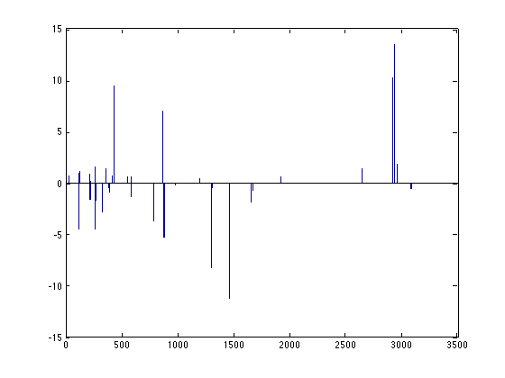
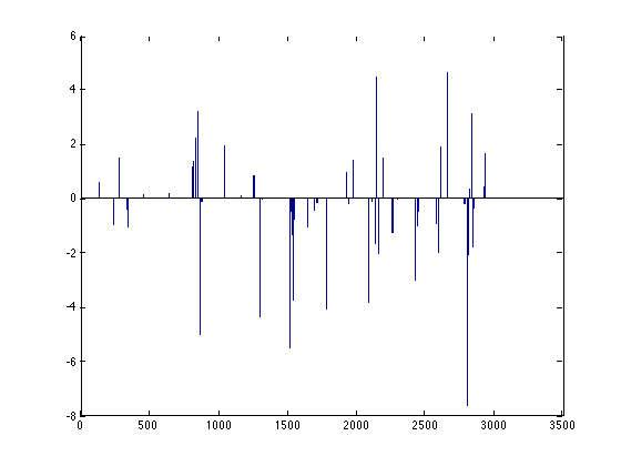
The sparse solution is returned in the model.weights field:

bar(m.model.weights);

Note however that directly finding the solution for a small L1 value can be numerically unstable. It's better to approximate this solution using small decreases in the L1 value. Furthermore, typically, the value of L1 is unknown and one wants to find such a value. This is where the gridsearch comes into play. We first generate a suitable regularization path (values of L1) to follow using a helper function

v = dml.graphnet.lambdapath(X,Y,'binomial',50,1e-2);

and then we use it in a gridsearch

m = dml.gridsearch('validator',dml.crossvalidator('type','split','stat','accuracy','mva',dml.graphnet('family','binomial','restart',false)),'vars','L1','vals',v);
tic; m = m.train(X,Y); toc

Elapsed time is 12.409168 seconds.

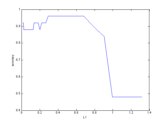
In order to see how performance changes as a function of L1, we can use the following code:

plot(m.configs,m.outcome); xlabel('L1'); ylabel('accuracy')

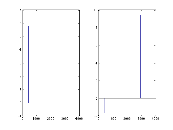
The associated configuration of parameter values is used to retrain the model on all data. This model can be accessed using the m.model field. Note that this model can differ from the model(s) obtained using crossvalidation since all data is used:

subplot(1,2,1); bar(m.models{m.optimum}.weights);
subplot(1,2,2); bar(m.model.weights);

The same results can be achieved using dml.glmnet. However, here the regularization term is a bit different:

$\lambda( (1-\alpha) \frac{1}{2}||\beta||^2_2 + \alpha ||\beta||_1 )$

Furthermore, the cross-validation and determination of the regularization path is done automatically inside the model. We can call this code as follows:

m = dml.enet;
tic; m = m.train(X,Y); toc;
close; bar(m.model.weights);

Elapsed time is 0.926965 seconds.

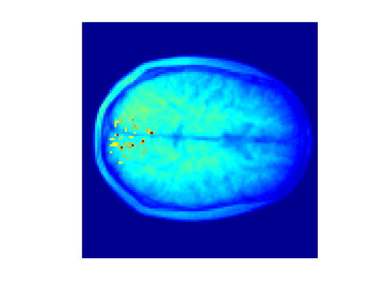
We can plot the contributions to the decoding back to brain space as follows:

M=mask; M(M) = m.model.weights;
imagesc(1e4*mean(abs(M),3)+mean(structural,3)); axis off; axis square;

Contents

Examples

Elastic net regression